# -*- coding: utf-8 -*-
# ---
# jupyter:
# jupytext:
# formats: ipynb,py:percent
# text_representation:
# extension: .py
# format_name: percent
# format_version: '1.3'
# jupytext_version: 1.13.0
# kernelspec:
# display_name: Python 3 (ipykernel)
# language: python
# name: python3
# ---
# %% [markdown] id="SX7UC-8jTsp7" tags=[]
#
# The Annotated Transformer
#
#
#
# Attention is All You Need
#
#
#
#  #
# * *v2022: Austin Huang, Suraj Subramanian, Jonathan Sum, Khalid Almubarak,
# and Stella Biderman.*
# * *[Original](https://nlp.seas.harvard.edu/2018/04/03/attention.html):
# [Sasha Rush](http://rush-nlp.com/).*
#
#
# The Transformer has been on a lot of
# people's minds over the last
year five years.
# This post presents an annotated version of the paper in the
# form of a line-by-line implementation. It reorders and deletes
# some sections from the original paper and adds comments
# throughout. This document itself is a working notebook, and should
# be a completely usable implementation.
# Code is available
# [here](https://github.com/harvardnlp/annotated-transformer/).
#
# %% [markdown] id="RSntDwKhTsp-"
# Table of Contents
#
# %% [markdown] id="BhmOhn9lTsp8"
# # Prelims
#
# Skip
# %% id="NwClcbH6Tsp8"
# # !pip install -r requirements.txt
# %% id="NwClcbH6Tsp8"
# # Uncomment for colab
# #
# # !pip install -q torchdata==0.3.0 torchtext==0.12 spacy==3.2 altair GPUtil
# # !python -m spacy download de_core_news_sm
# # !python -m spacy download en_core_web_sm
# %% id="v1-1MX6oTsp9"
import os
from os.path import exists
import torch
import torch.nn as nn
from torch.nn.functional import log_softmax, pad
import math
import copy
import time
from torch.optim.lr_scheduler import LambdaLR
import pandas as pd
import altair as alt
from torchtext.data.functional import to_map_style_dataset
from torch.utils.data import DataLoader
from torchtext.vocab import build_vocab_from_iterator
import torchtext.datasets as datasets
import spacy
import GPUtil
import warnings
from torch.utils.data.distributed import DistributedSampler
import torch.distributed as dist
import torch.multiprocessing as mp
from torch.nn.parallel import DistributedDataParallel as DDP
# Set to False to skip notebook execution (e.g. for debugging)
warnings.filterwarnings("ignore")
RUN_EXAMPLES = True
# %%
# Some convenience helper functions used throughout the notebook
def is_interactive_notebook():
return __name__ == "__main__"
def show_example(fn, args=[]):
if __name__ == "__main__" and RUN_EXAMPLES:
return fn(*args)
def execute_example(fn, args=[]):
if __name__ == "__main__" and RUN_EXAMPLES:
fn(*args)
class DummyOptimizer(torch.optim.Optimizer):
def __init__(self):
self.param_groups = [{"lr": 0}]
None
def step(self):
None
def zero_grad(self, set_to_none=False):
None
class DummyScheduler:
def step(self):
None
# %% [markdown] id="jx49WRyfTsp-"
# > My comments are blockquoted. The main text is all from the paper itself.
# %% [markdown] id="7phVeWghTsp_"
# # Background
# %% [markdown] id="83ZDS91dTsqA"
#
# The goal of reducing sequential computation also forms the
# foundation of the Extended Neural GPU, ByteNet and ConvS2S, all of
# which use convolutional neural networks as basic building block,
# computing hidden representations in parallel for all input and
# output positions. In these models, the number of operations required
# to relate signals from two arbitrary input or output positions grows
# in the distance between positions, linearly for ConvS2S and
# logarithmically for ByteNet. This makes it more difficult to learn
# dependencies between distant positions. In the Transformer this is
# reduced to a constant number of operations, albeit at the cost of
# reduced effective resolution due to averaging attention-weighted
# positions, an effect we counteract with Multi-Head Attention.
#
# Self-attention, sometimes called intra-attention is an attention
# mechanism relating different positions of a single sequence in order
# to compute a representation of the sequence. Self-attention has been
# used successfully in a variety of tasks including reading
# comprehension, abstractive summarization, textual entailment and
# learning task-independent sentence representations. End-to-end
# memory networks are based on a recurrent attention mechanism instead
# of sequencealigned recurrence and have been shown to perform well on
# simple-language question answering and language modeling tasks.
#
# To the best of our knowledge, however, the Transformer is the first
# transduction model relying entirely on self-attention to compute
# representations of its input and output without using sequence
# aligned RNNs or convolution.
# %% [markdown]
# # Part 1: Model Architecture
# %% [markdown] id="pFrPajezTsqB"
# # Model Architecture
# %% [markdown] id="ReuU_h-fTsqB"
#
# Most competitive neural sequence transduction models have an
# encoder-decoder structure
# [(cite)](https://arxiv.org/abs/1409.0473). Here, the encoder maps an
# input sequence of symbol representations $(x_1, ..., x_n)$ to a
# sequence of continuous representations $\mathbf{z} = (z_1, ...,
# z_n)$. Given $\mathbf{z}$, the decoder then generates an output
# sequence $(y_1,...,y_m)$ of symbols one element at a time. At each
# step the model is auto-regressive
# [(cite)](https://arxiv.org/abs/1308.0850), consuming the previously
# generated symbols as additional input when generating the next.
# %% id="k0XGXhzRTsqB"
class EncoderDecoder(nn.Module):
"""
A standard Encoder-Decoder architecture. Base for this and many
other models.
"""
def __init__(self, encoder, decoder, src_embed, tgt_embed, generator):
super(EncoderDecoder, self).__init__()
self.encoder = encoder
self.decoder = decoder
self.src_embed = src_embed
self.tgt_embed = tgt_embed
self.generator = generator
def forward(self, src, tgt, src_mask, tgt_mask):
"Take in and process masked src and target sequences."
return self.decode(self.encode(src, src_mask), src_mask, tgt, tgt_mask)
def encode(self, src, src_mask):
return self.encoder(self.src_embed(src), src_mask)
def decode(self, memory, src_mask, tgt, tgt_mask):
return self.decoder(self.tgt_embed(tgt), memory, src_mask, tgt_mask)
# %% id="NKGoH2RsTsqC"
class Generator(nn.Module):
"Define standard linear + softmax generation step."
def __init__(self, d_model, vocab):
super(Generator, self).__init__()
self.proj = nn.Linear(d_model, vocab)
def forward(self, x):
return log_softmax(self.proj(x), dim=-1)
# %% [markdown] id="mOoEnF_jTsqC"
#
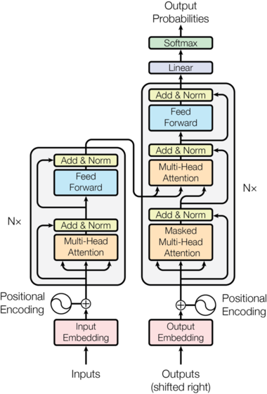
# The Transformer follows this overall architecture using stacked
# self-attention and point-wise, fully connected layers for both the
# encoder and decoder, shown in the left and right halves of Figure 1,
# respectively.
# %% [markdown] id="oredWloYTsqC"
# 
# %% [markdown] id="bh092NZBTsqD"
# ## Encoder and Decoder Stacks
#
# ### Encoder
#
# The encoder is composed of a stack of $N=6$ identical layers.
# %% id="2gxTApUYTsqD"
def clones(module, N):
"Produce N identical layers."
return nn.ModuleList([copy.deepcopy(module) for _ in range(N)])
# %% id="xqVTz9MkTsqD"
class Encoder(nn.Module):
"Core encoder is a stack of N layers"
def __init__(self, layer, N):
super(Encoder, self).__init__()
self.layers = clones(layer, N)
self.norm = LayerNorm(layer.size)
def forward(self, x, mask):
"Pass the input (and mask) through each layer in turn."
for layer in self.layers:
x = layer(x, mask)
return self.norm(x)
# %% [markdown] id="GjAKgjGwTsqD"
#
# We employ a residual connection
# [(cite)](https://arxiv.org/abs/1512.03385) around each of the two
# sub-layers, followed by layer normalization
# [(cite)](https://arxiv.org/abs/1607.06450).
# %% id="3jKa_prZTsqE"
class LayerNorm(nn.Module):
"Construct a layernorm module (See citation for details)."
def __init__(self, features, eps=1e-6):
super(LayerNorm, self).__init__()
self.a_2 = nn.Parameter(torch.ones(features))
self.b_2 = nn.Parameter(torch.zeros(features))
self.eps = eps
def forward(self, x):
mean = x.mean(-1, keepdim=True)
std = x.std(-1, keepdim=True)
return self.a_2 * (x - mean) / (std + self.eps) + self.b_2
# %% [markdown] id="nXSJ3QYmTsqE"
#
# That is, the output of each sub-layer is $\mathrm{LayerNorm}(x +
# \mathrm{Sublayer}(x))$, where $\mathrm{Sublayer}(x)$ is the function
# implemented by the sub-layer itself. We apply dropout
# [(cite)](http://jmlr.org/papers/v15/srivastava14a.html) to the
# output of each sub-layer, before it is added to the sub-layer input
# and normalized.
#
# To facilitate these residual connections, all sub-layers in the
# model, as well as the embedding layers, produce outputs of dimension
# $d_{\text{model}}=512$.
# %% id="U1P7zI0eTsqE"
class SublayerConnection(nn.Module):
"""
A residual connection followed by a layer norm.
Note for code simplicity the norm is first as opposed to last.
"""
def __init__(self, size, dropout):
super(SublayerConnection, self).__init__()
self.norm = LayerNorm(size)
self.dropout = nn.Dropout(dropout)
def forward(self, x, sublayer):
"Apply residual connection to any sublayer with the same size."
return x + self.dropout(sublayer(self.norm(x)))
# %% [markdown] id="ML6oDlEqTsqE"
#
# Each layer has two sub-layers. The first is a multi-head
# self-attention mechanism, and the second is a simple, position-wise
# fully connected feed-forward network.
# %% id="qYkUFr6GTsqE"
class EncoderLayer(nn.Module):
"Encoder is made up of self-attn and feed forward (defined below)"
def __init__(self, size, self_attn, feed_forward, dropout):
super(EncoderLayer, self).__init__()
self.self_attn = self_attn
self.feed_forward = feed_forward
self.sublayer = clones(SublayerConnection(size, dropout), 2)
self.size = size
def forward(self, x, mask):
"Follow Figure 1 (left) for connections."
x = self.sublayer[0](x, lambda x: self.self_attn(x, x, x, mask))
return self.sublayer[1](x, self.feed_forward)
# %% [markdown] id="7ecOQIhkTsqF"
# ### Decoder
#
# The decoder is also composed of a stack of $N=6$ identical layers.
#
# %%
class Decoder(nn.Module):
"Generic N layer decoder with masking."
def __init__(self, layer, N):
super(Decoder, self).__init__()
self.layers = clones(layer, N)
self.norm = LayerNorm(layer.size)
def forward(self, x, memory, src_mask, tgt_mask):
for layer in self.layers:
x = layer(x, memory, src_mask, tgt_mask)
return self.norm(x)
# %% [markdown] id="dXlCB12pTsqF"
#
# In addition to the two sub-layers in each encoder layer, the decoder
# inserts a third sub-layer, which performs multi-head attention over
# the output of the encoder stack. Similar to the encoder, we employ
# residual connections around each of the sub-layers, followed by
# layer normalization.
# %% id="M2hA1xFQTsqF"
class DecoderLayer(nn.Module):
"Decoder is made of self-attn, src-attn, and feed forward (defined below)"
def __init__(self, size, self_attn, src_attn, feed_forward, dropout):
super(DecoderLayer, self).__init__()
self.size = size
self.self_attn = self_attn
self.src_attn = src_attn
self.feed_forward = feed_forward
self.sublayer = clones(SublayerConnection(size, dropout), 3)
def forward(self, x, memory, src_mask, tgt_mask):
"Follow Figure 1 (right) for connections."
m = memory
x = self.sublayer[0](x, lambda x: self.self_attn(x, x, x, tgt_mask))
x = self.sublayer[1](x, lambda x: self.src_attn(x, m, m, src_mask))
return self.sublayer[2](x, self.feed_forward)
# %% [markdown] id="FZz5rLl4TsqF"
#
# We also modify the self-attention sub-layer in the decoder stack to
# prevent positions from attending to subsequent positions. This
# masking, combined with fact that the output embeddings are offset by
# one position, ensures that the predictions for position $i$ can
# depend only on the known outputs at positions less than $i$.
# %% id="QN98O2l3TsqF"
def subsequent_mask(size):
"Mask out subsequent positions."
attn_shape = (1, size, size)
subsequent_mask = torch.triu(torch.ones(attn_shape), diagonal=1).type(
torch.uint8
)
return subsequent_mask == 0
# %% [markdown] id="Vg_f_w-PTsqG"
#
# > Below the attention mask shows the position each tgt word (row) is
# > allowed to look at (column). Words are blocked for attending to
# > future words during training.
# %% id="ht_FtgYAokC4"
def example_mask():
LS_data = pd.concat(
[
pd.DataFrame(
{
"Subsequent Mask": subsequent_mask(20)[0][x, y].flatten(),
"Window": y,
"Masking": x,
}
)
for y in range(20)
for x in range(20)
]
)
return (
alt.Chart(LS_data)
.mark_rect()
.properties(height=250, width=250)
.encode(
alt.X("Window:O"),
alt.Y("Masking:O"),
alt.Color("Subsequent Mask:Q", scale=alt.Scale(scheme="viridis")),
)
.interactive()
)
show_example(example_mask)
# %% [markdown] id="Qto_yg7BTsqG"
# ### Attention
#
# An attention function can be described as mapping a query and a set
# of key-value pairs to an output, where the query, keys, values, and
# output are all vectors. The output is computed as a weighted sum of
# the values, where the weight assigned to each value is computed by a
# compatibility function of the query with the corresponding key.
#
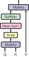
# We call our particular attention "Scaled Dot-Product Attention".
# The input consists of queries and keys of dimension $d_k$, and
# values of dimension $d_v$. We compute the dot products of the query
# with all keys, divide each by $\sqrt{d_k}$, and apply a softmax
# function to obtain the weights on the values.
#
#
#
# 
# %% [markdown] id="EYJLWk6cTsqG"
#
# In practice, we compute the attention function on a set of queries
# simultaneously, packed together into a matrix $Q$. The keys and
# values are also packed together into matrices $K$ and $V$. We
# compute the matrix of outputs as:
#
# $$
# \mathrm{Attention}(Q, K, V) = \mathrm{softmax}(\frac{QK^T}{\sqrt{d_k}})V
# $$
# %% id="qsoVxS5yTsqG"
def attention(query, key, value, mask=None, dropout=None):
"Compute 'Scaled Dot Product Attention'"
d_k = query.size(-1)
scores = torch.matmul(query, key.transpose(-2, -1)) / math.sqrt(d_k)
if mask is not None:
scores = scores.masked_fill(mask == 0, -1e9)
p_attn = scores.softmax(dim=-1)
if dropout is not None:
p_attn = dropout(p_attn)
return torch.matmul(p_attn, value), p_attn
# %% [markdown] id="jUkpwu8kTsqG"
#
# The two most commonly used attention functions are additive
# attention [(cite)](https://arxiv.org/abs/1409.0473), and dot-product
# (multiplicative) attention. Dot-product attention is identical to
# our algorithm, except for the scaling factor of
# $\frac{1}{\sqrt{d_k}}$. Additive attention computes the
# compatibility function using a feed-forward network with a single
# hidden layer. While the two are similar in theoretical complexity,
# dot-product attention is much faster and more space-efficient in
# practice, since it can be implemented using highly optimized matrix
# multiplication code.
#
#
# While for small values of $d_k$ the two mechanisms perform
# similarly, additive attention outperforms dot product attention
# without scaling for larger values of $d_k$
# [(cite)](https://arxiv.org/abs/1703.03906). We suspect that for
# large values of $d_k$, the dot products grow large in magnitude,
# pushing the softmax function into regions where it has extremely
# small gradients (To illustrate why the dot products get large,
# assume that the components of $q$ and $k$ are independent random
# variables with mean $0$ and variance $1$. Then their dot product,
# $q \cdot k = \sum_{i=1}^{d_k} q_ik_i$, has mean $0$ and variance
# $d_k$.). To counteract this effect, we scale the dot products by
# $\frac{1}{\sqrt{d_k}}$.
#
#
# %% [markdown] id="bS1FszhVTsqG"
# 
# %% [markdown] id="TNtVyZ-pTsqH"
#
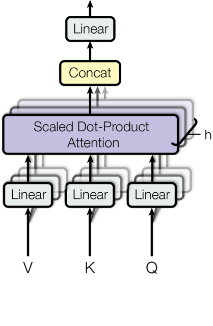
# Multi-head attention allows the model to jointly attend to
# information from different representation subspaces at different
# positions. With a single attention head, averaging inhibits this.
#
# $$
# \mathrm{MultiHead}(Q, K, V) =
# \mathrm{Concat}(\mathrm{head_1}, ..., \mathrm{head_h})W^O \\
# \text{where}~\mathrm{head_i} = \mathrm{Attention}(QW^Q_i, KW^K_i, VW^V_i)
# $$
#
# Where the projections are parameter matrices $W^Q_i \in
# \mathbb{R}^{d_{\text{model}} \times d_k}$, $W^K_i \in
# \mathbb{R}^{d_{\text{model}} \times d_k}$, $W^V_i \in
# \mathbb{R}^{d_{\text{model}} \times d_v}$ and $W^O \in
# \mathbb{R}^{hd_v \times d_{\text{model}}}$.
#
# In this work we employ $h=8$ parallel attention layers, or
# heads. For each of these we use $d_k=d_v=d_{\text{model}}/h=64$. Due
# to the reduced dimension of each head, the total computational cost
# is similar to that of single-head attention with full
# dimensionality.
# %% id="D2LBMKCQTsqH"
class MultiHeadedAttention(nn.Module):
def __init__(self, h, d_model, dropout=0.1):
"Take in model size and number of heads."
super(MultiHeadedAttention, self).__init__()
assert d_model % h == 0
# We assume d_v always equals d_k
self.d_k = d_model // h
self.h = h
self.linears = clones(nn.Linear(d_model, d_model), 4)
self.attn = None
self.dropout = nn.Dropout(p=dropout)
def forward(self, query, key, value, mask=None):
"Implements Figure 2"
if mask is not None:
# Same mask applied to all h heads.
mask = mask.unsqueeze(1)
nbatches = query.size(0)
# 1) Do all the linear projections in batch from d_model => h x d_k
query, key, value = [
lin(x).view(nbatches, -1, self.h, self.d_k).transpose(1, 2)
for lin, x in zip(self.linears, (query, key, value))
]
# 2) Apply attention on all the projected vectors in batch.
x, self.attn = attention(
query, key, value, mask=mask, dropout=self.dropout
)
# 3) "Concat" using a view and apply a final linear.
x = (
x.transpose(1, 2)
.contiguous()
.view(nbatches, -1, self.h * self.d_k)
)
del query
del key
del value
return self.linears[-1](x)
# %% [markdown] id="EDRba3J3TsqH"
# ### Applications of Attention in our Model
#
# The Transformer uses multi-head attention in three different ways:
# 1) In "encoder-decoder attention" layers, the queries come from the
# previous decoder layer, and the memory keys and values come from the
# output of the encoder. This allows every position in the decoder to
# attend over all positions in the input sequence. This mimics the
# typical encoder-decoder attention mechanisms in sequence-to-sequence
# models such as [(cite)](https://arxiv.org/abs/1609.08144).
#
#
# 2) The encoder contains self-attention layers. In a self-attention
# layer all of the keys, values and queries come from the same place,
# in this case, the output of the previous layer in the encoder. Each
# position in the encoder can attend to all positions in the previous
# layer of the encoder.
#
#
# 3) Similarly, self-attention layers in the decoder allow each
# position in the decoder to attend to all positions in the decoder up
# to and including that position. We need to prevent leftward
# information flow in the decoder to preserve the auto-regressive
# property. We implement this inside of scaled dot-product attention
# by masking out (setting to $-\infty$) all values in the input of the
# softmax which correspond to illegal connections.
# %% [markdown] id="M-en97_GTsqH"
# ## Position-wise Feed-Forward Networks
#
# In addition to attention sub-layers, each of the layers in our
# encoder and decoder contains a fully connected feed-forward network,
# which is applied to each position separately and identically. This
# consists of two linear transformations with a ReLU activation in
# between.
#
# $$\mathrm{FFN}(x)=\max(0, xW_1 + b_1) W_2 + b_2$$
#
# While the linear transformations are the same across different
# positions, they use different parameters from layer to
# layer. Another way of describing this is as two convolutions with
# kernel size 1. The dimensionality of input and output is
# $d_{\text{model}}=512$, and the inner-layer has dimensionality
# $d_{ff}=2048$.
# %% id="6HHCemCxTsqH"
class PositionwiseFeedForward(nn.Module):
"Implements FFN equation."
def __init__(self, d_model, d_ff, dropout=0.1):
super(PositionwiseFeedForward, self).__init__()
self.w_1 = nn.Linear(d_model, d_ff)
self.w_2 = nn.Linear(d_ff, d_model)
self.dropout = nn.Dropout(dropout)
def forward(self, x):
return self.w_2(self.dropout(self.w_1(x).relu()))
# %% [markdown] id="dR1YM520TsqH"
# ## Embeddings and Softmax
#
# Similarly to other sequence transduction models, we use learned
# embeddings to convert the input tokens and output tokens to vectors
# of dimension $d_{\text{model}}$. We also use the usual learned
# linear transformation and softmax function to convert the decoder
# output to predicted next-token probabilities. In our model, we
# share the same weight matrix between the two embedding layers and
# the pre-softmax linear transformation, similar to
# [(cite)](https://arxiv.org/abs/1608.05859). In the embedding layers,
# we multiply those weights by $\sqrt{d_{\text{model}}}$.
# %% id="pyrChq9qTsqH"
class Embeddings(nn.Module):
def __init__(self, d_model, vocab):
super(Embeddings, self).__init__()
self.lut = nn.Embedding(vocab, d_model)
self.d_model = d_model
def forward(self, x):
return self.lut(x) * math.sqrt(self.d_model)
# %% [markdown] id="vOkdui-cTsqH"
# ## Positional Encoding
#
# Since our model contains no recurrence and no convolution, in order
# for the model to make use of the order of the sequence, we must
# inject some information about the relative or absolute position of
# the tokens in the sequence. To this end, we add "positional
# encodings" to the input embeddings at the bottoms of the encoder and
# decoder stacks. The positional encodings have the same dimension
# $d_{\text{model}}$ as the embeddings, so that the two can be summed.
# There are many choices of positional encodings, learned and fixed
# [(cite)](https://arxiv.org/pdf/1705.03122.pdf).
#
# In this work, we use sine and cosine functions of different frequencies:
#
# $$PE_{(pos,2i)} = \sin(pos / 10000^{2i/d_{\text{model}}})$$
#
# $$PE_{(pos,2i+1)} = \cos(pos / 10000^{2i/d_{\text{model}}})$$
#
# where $pos$ is the position and $i$ is the dimension. That is, each
# dimension of the positional encoding corresponds to a sinusoid. The
# wavelengths form a geometric progression from $2\pi$ to $10000 \cdot
# 2\pi$. We chose this function because we hypothesized it would
# allow the model to easily learn to attend by relative positions,
# since for any fixed offset $k$, $PE_{pos+k}$ can be represented as a
# linear function of $PE_{pos}$.
#
# In addition, we apply dropout to the sums of the embeddings and the
# positional encodings in both the encoder and decoder stacks. For
# the base model, we use a rate of $P_{drop}=0.1$.
#
#
# %% id="zaHGD4yJTsqH"
class PositionalEncoding(nn.Module):
"Implement the PE function."
def __init__(self, d_model, dropout, max_len=5000):
super(PositionalEncoding, self).__init__()
self.dropout = nn.Dropout(p=dropout)
# Compute the positional encodings once in log space.
pe = torch.zeros(max_len, d_model)
position = torch.arange(0, max_len).unsqueeze(1)
div_term = torch.exp(
torch.arange(0, d_model, 2) * -(math.log(10000.0) / d_model)
)
pe[:, 0::2] = torch.sin(position * div_term)
pe[:, 1::2] = torch.cos(position * div_term)
pe = pe.unsqueeze(0)
self.register_buffer("pe", pe)
def forward(self, x):
x = x + self.pe[:, : x.size(1)].requires_grad_(False)
return self.dropout(x)
# %% [markdown] id="EfHacTJLTsqH"
#
# > Below the positional encoding will add in a sine wave based on
# > position. The frequency and offset of the wave is different for
# > each dimension.
# %% id="rnvHk_1QokC6" type="example"
def example_positional():
pe = PositionalEncoding(20, 0)
y = pe.forward(torch.zeros(1, 100, 20))
data = pd.concat(
[
pd.DataFrame(
{
"embedding": y[0, :, dim],
"dimension": dim,
"position": list(range(100)),
}
)
for dim in [4, 5, 6, 7]
]
)
return (
alt.Chart(data)
.mark_line()
.properties(width=800)
.encode(x="position", y="embedding", color="dimension:N")
.interactive()
)
show_example(example_positional)
# %% [markdown] id="g8rZNCrzTsqI"
#
# We also experimented with using learned positional embeddings
# [(cite)](https://arxiv.org/pdf/1705.03122.pdf) instead, and found
# that the two versions produced nearly identical results. We chose
# the sinusoidal version because it may allow the model to extrapolate
# to sequence lengths longer than the ones encountered during
# training.
# %% [markdown] id="iwNKCzlyTsqI"
# ## Full Model
#
# > Here we define a function from hyperparameters to a full model.
# %% id="mPe1ES0UTsqI"
def make_model(
src_vocab, tgt_vocab, N=6, d_model=512, d_ff=2048, h=8, dropout=0.1
):
"Helper: Construct a model from hyperparameters."
c = copy.deepcopy
attn = MultiHeadedAttention(h, d_model)
ff = PositionwiseFeedForward(d_model, d_ff, dropout)
position = PositionalEncoding(d_model, dropout)
model = EncoderDecoder(
Encoder(EncoderLayer(d_model, c(attn), c(ff), dropout), N),
Decoder(DecoderLayer(d_model, c(attn), c(attn), c(ff), dropout), N),
nn.Sequential(Embeddings(d_model, src_vocab), c(position)),
nn.Sequential(Embeddings(d_model, tgt_vocab), c(position)),
Generator(d_model, tgt_vocab),
)
# This was important from their code.
# Initialize parameters with Glorot / fan_avg.
for p in model.parameters():
if p.dim() > 1:
nn.init.xavier_uniform_(p)
return model
# %% [markdown]
# ## Inference:
#
# > Here we make a forward step to generate a prediction of the
# model. We try to use our transformer to memorize the input. As you
# will see the output is randomly generated due to the fact that the
# model is not trained yet. In the next tutorial we will build the
# training function and try to train our model to memorize the numbers
# from 1 to 10.
# %%
def inference_test():
test_model = make_model(11, 11, 2)
test_model.eval()
src = torch.LongTensor([[1, 2, 3, 4, 5, 6, 7, 8, 9, 10]])
src_mask = torch.ones(1, 1, 10)
memory = test_model.encode(src, src_mask)
ys = torch.zeros(1, 1).type_as(src)
for i in range(9):
out = test_model.decode(
memory, src_mask, ys, subsequent_mask(ys.size(1)).type_as(src.data)
)
prob = test_model.generator(out[:, -1])
_, next_word = torch.max(prob, dim=1)
next_word = next_word.data[0]
ys = torch.cat(
[ys, torch.empty(1, 1).type_as(src.data).fill_(next_word)], dim=1
)
print("Example Untrained Model Prediction:", ys)
def run_tests():
for _ in range(10):
inference_test()
show_example(run_tests)
# %% [markdown]
# # Part 2: Model Training
# %% [markdown] id="05s6oT9fTsqI"
# # Training
#
# This section describes the training regime for our models.
# %% [markdown] id="fTxlofs4TsqI"
#
# > We stop for a quick interlude to introduce some of the tools
# > needed to train a standard encoder decoder model. First we define a
# > batch object that holds the src and target sentences for training,
# > as well as constructing the masks.
# %% [markdown] id="G7SkCenXTsqI"
# ## Batches and Masking
# %%
class Batch:
"""Object for holding a batch of data with mask during training."""
def __init__(self, src, tgt=None, pad=2): # 2 =
self.src = src
self.src_mask = (src != pad).unsqueeze(-2)
if tgt is not None:
self.tgt = tgt[:, :-1]
self.tgt_y = tgt[:, 1:]
self.tgt_mask = self.make_std_mask(self.tgt, pad)
self.ntokens = (self.tgt_y != pad).data.sum()
@staticmethod
def make_std_mask(tgt, pad):
"Create a mask to hide padding and future words."
tgt_mask = (tgt != pad).unsqueeze(-2)
tgt_mask = tgt_mask & subsequent_mask(tgt.size(-1)).type_as(
tgt_mask.data
)
return tgt_mask
# %% [markdown] id="cKkw5GjLTsqI"
#
# > Next we create a generic training and scoring function to keep
# > track of loss. We pass in a generic loss compute function that
# > also handles parameter updates.
# %% [markdown] id="Q8zzeUc0TsqJ"
# ## Training Loop
# %%
class TrainState:
"""Track number of steps, examples, and tokens processed"""
step: int = 0 # Steps in the current epoch
accum_step: int = 0 # Number of gradient accumulation steps
samples: int = 0 # total # of examples used
tokens: int = 0 # total # of tokens processed
# %% id="2HAZD3hiTsqJ"
def run_epoch(
data_iter,
model,
loss_compute,
optimizer,
scheduler,
mode="train",
accum_iter=1,
train_state=TrainState(),
):
"""Train a single epoch"""
start = time.time()
total_tokens = 0
total_loss = 0
tokens = 0
n_accum = 0
for i, batch in enumerate(data_iter):
out = model.forward(
batch.src, batch.tgt, batch.src_mask, batch.tgt_mask
)
loss, loss_node = loss_compute(out, batch.tgt_y, batch.ntokens)
# loss_node = loss_node / accum_iter
if mode == "train" or mode == "train+log":
loss_node.backward()
train_state.step += 1
train_state.samples += batch.src.shape[0]
train_state.tokens += batch.ntokens
if i % accum_iter == 0:
optimizer.step()
optimizer.zero_grad(set_to_none=True)
n_accum += 1
train_state.accum_step += 1
scheduler.step()
total_loss += loss
total_tokens += batch.ntokens
tokens += batch.ntokens
if i % 40 == 1 and (mode == "train" or mode == "train+log"):
lr = optimizer.param_groups[0]["lr"]
elapsed = time.time() - start
print(
(
"Epoch Step: %6d | Accumulation Step: %3d | Loss: %6.2f "
+ "| Tokens / Sec: %7.1f | Learning Rate: %6.1e"
)
% (i, n_accum, loss / batch.ntokens, tokens / elapsed, lr)
)
start = time.time()
tokens = 0
del loss
del loss_node
return total_loss / total_tokens, train_state
# %% [markdown] id="aB1IF0foTsqJ"
# ## Training Data and Batching
#
# We trained on the standard WMT 2014 English-German dataset
# consisting of about 4.5 million sentence pairs. Sentences were
# encoded using byte-pair encoding, which has a shared source-target
# vocabulary of about 37000 tokens. For English-French, we used the
# significantly larger WMT 2014 English-French dataset consisting of
# 36M sentences and split tokens into a 32000 word-piece vocabulary.
#
#
# Sentence pairs were batched together by approximate sequence length.
# Each training batch contained a set of sentence pairs containing
# approximately 25000 source tokens and 25000 target tokens.
# %% [markdown] id="F1mTQatiTsqJ" jp-MarkdownHeadingCollapsed=true tags=[]
# ## Hardware and Schedule
#
# We trained our models on one machine with 8 NVIDIA P100 GPUs. For
# our base models using the hyperparameters described throughout the
# paper, each training step took about 0.4 seconds. We trained the
# base models for a total of 100,000 steps or 12 hours. For our big
# models, step time was 1.0 seconds. The big models were trained for
# 300,000 steps (3.5 days).
# %% [markdown] id="-utZeuGcTsqJ"
# ## Optimizer
#
# We used the Adam optimizer [(cite)](https://arxiv.org/abs/1412.6980)
# with $\beta_1=0.9$, $\beta_2=0.98$ and $\epsilon=10^{-9}$. We
# varied the learning rate over the course of training, according to
# the formula:
#
# $$
# lrate = d_{\text{model}}^{-0.5} \cdot
# \min({step\_num}^{-0.5},
# {step\_num} \cdot {warmup\_steps}^{-1.5})
# $$
#
# This corresponds to increasing the learning rate linearly for the
# first $warmup\_steps$ training steps, and decreasing it thereafter
# proportionally to the inverse square root of the step number. We
# used $warmup\_steps=4000$.
# %% [markdown] id="39FbYnt-TsqJ"
#
# > Note: This part is very important. Need to train with this setup
# > of the model.
# %% [markdown] id="hlbojFkjTsqJ"
#
# > Example of the curves of this model for different model sizes and
# > for optimization hyperparameters.
# %% id="zUz3PdAnVg4o"
def rate(step, model_size, factor, warmup):
"""
we have to default the step to 1 for LambdaLR function
to avoid zero raising to negative power.
"""
if step == 0:
step = 1
return factor * (
model_size ** (-0.5) * min(step ** (-0.5), step * warmup ** (-1.5))
)
# %% id="l1bnrlnSV8J5" tags=[]
def example_learning_schedule():
opts = [
[512, 1, 4000], # example 1
[512, 1, 8000], # example 2
[256, 1, 4000], # example 3
]
dummy_model = torch.nn.Linear(1, 1)
learning_rates = []
# we have 3 examples in opts list.
for idx, example in enumerate(opts):
# run 20000 epoch for each example
optimizer = torch.optim.Adam(
dummy_model.parameters(), lr=1, betas=(0.9, 0.98), eps=1e-9
)
lr_scheduler = LambdaLR(
optimizer=optimizer, lr_lambda=lambda step: rate(step, *example)
)
tmp = []
# take 20K dummy training steps, save the learning rate at each step
for step in range(20000):
tmp.append(optimizer.param_groups[0]["lr"])
optimizer.step()
lr_scheduler.step()
learning_rates.append(tmp)
learning_rates = torch.tensor(learning_rates)
# Enable altair to handle more than 5000 rows
alt.data_transformers.disable_max_rows()
opts_data = pd.concat(
[
pd.DataFrame(
{
"Learning Rate": learning_rates[warmup_idx, :],
"model_size:warmup": ["512:4000", "512:8000", "256:4000"][
warmup_idx
],
"step": range(20000),
}
)
for warmup_idx in [0, 1, 2]
]
)
return (
alt.Chart(opts_data)
.mark_line()
.properties(width=600)
.encode(x="step", y="Learning Rate", color="model_size:warmup:N")
.interactive()
)
example_learning_schedule()
# %% [markdown] id="7T1uD15VTsqK"
# ## Regularization
#
# ### Label Smoothing
#
# During training, we employed label smoothing of value
# $\epsilon_{ls}=0.1$ [(cite)](https://arxiv.org/abs/1512.00567).
# This hurts perplexity, as the model learns to be more unsure, but
# improves accuracy and BLEU score.
# %% [markdown] id="kNoAVD8bTsqK"
#
# > We implement label smoothing using the KL div loss. Instead of
# > using a one-hot target distribution, we create a distribution that
# > has `confidence` of the correct word and the rest of the
# > `smoothing` mass distributed throughout the vocabulary.
# %% id="shU2GyiETsqK"
class LabelSmoothing(nn.Module):
"Implement label smoothing."
def __init__(self, size, padding_idx, smoothing=0.0):
super(LabelSmoothing, self).__init__()
self.criterion = nn.KLDivLoss(reduction="sum")
self.padding_idx = padding_idx
self.confidence = 1.0 - smoothing
self.smoothing = smoothing
self.size = size
self.true_dist = None
def forward(self, x, target):
assert x.size(1) == self.size
true_dist = x.data.clone()
true_dist.fill_(self.smoothing / (self.size - 2))
true_dist.scatter_(1, target.data.unsqueeze(1), self.confidence)
true_dist[:, self.padding_idx] = 0
mask = torch.nonzero(target.data == self.padding_idx)
if mask.dim() > 0:
true_dist.index_fill_(0, mask.squeeze(), 0.0)
self.true_dist = true_dist
return self.criterion(x, true_dist.clone().detach())
# %% [markdown] id="jCxUrlUyTsqK"
#
# > Here we can see an example of how the mass is distributed to the
# > words based on confidence.
# %% id="EZtKaaQNTsqK"
# Example of label smoothing.
def example_label_smoothing():
crit = LabelSmoothing(5, 0, 0.4)
predict = torch.FloatTensor(
[
[0, 0.2, 0.7, 0.1, 0],
[0, 0.2, 0.7, 0.1, 0],
[0, 0.2, 0.7, 0.1, 0],
[0, 0.2, 0.7, 0.1, 0],
[0, 0.2, 0.7, 0.1, 0],
]
)
crit(x=predict.log(), target=torch.LongTensor([2, 1, 0, 3, 3]))
LS_data = pd.concat(
[
pd.DataFrame(
{
"target distribution": crit.true_dist[x, y].flatten(),
"columns": y,
"rows": x,
}
)
for y in range(5)
for x in range(5)
]
)
return (
alt.Chart(LS_data)
.mark_rect(color="Blue", opacity=1)
.properties(height=200, width=200)
.encode(
alt.X("columns:O", title=None),
alt.Y("rows:O", title=None),
alt.Color(
"target distribution:Q", scale=alt.Scale(scheme="viridis")
),
)
.interactive()
)
show_example(example_label_smoothing)
# %% [markdown] id="CGM8J1veTsqK"
#
# > Label smoothing actually starts to penalize the model if it gets
# > very confident about a given choice.
# %% id="78EHzLP7TsqK"
def loss(x, crit):
d = x + 3 * 1
predict = torch.FloatTensor([[0, x / d, 1 / d, 1 / d, 1 / d]])
return crit(predict.log(), torch.LongTensor([1])).data
def penalization_visualization():
crit = LabelSmoothing(5, 0, 0.1)
loss_data = pd.DataFrame(
{
"Loss": [loss(x, crit) for x in range(1, 100)],
"Steps": list(range(99)),
}
).astype("float")
return (
alt.Chart(loss_data)
.mark_line()
.properties(width=350)
.encode(
x="Steps",
y="Loss",
)
.interactive()
)
show_example(penalization_visualization)
# %% [markdown] id="67lUqeLXTsqK"
# # A First Example
#
# > We can begin by trying out a simple copy-task. Given a random set
# > of input symbols from a small vocabulary, the goal is to generate
# > back those same symbols.
# %% [markdown] id="jJa-89_pTsqK"
# ## Synthetic Data
# %% id="g1aTxeqqTsqK"
def data_gen(V, batch_size, nbatches):
"Generate random data for a src-tgt copy task."
for i in range(nbatches):
data = torch.randint(1, V, size=(batch_size, 10))
data[:, 0] = 1
src = data.requires_grad_(False).clone().detach()
tgt = data.requires_grad_(False).clone().detach()
yield Batch(src, tgt, 0)
# %% [markdown] id="XTXwD9hUTsqK"
# ## Loss Computation
# %% id="3J8EJm87TsqK"
class SimpleLossCompute:
"A simple loss compute and train function."
def __init__(self, generator, criterion):
self.generator = generator
self.criterion = criterion
def __call__(self, x, y, norm):
x = self.generator(x)
sloss = (
self.criterion(
x.contiguous().view(-1, x.size(-1)), y.contiguous().view(-1)
)
/ norm
)
return sloss.data * norm, sloss
# %% [markdown] id="eDAI7ELUTsqL"
# ## Greedy Decoding
# %% [markdown] id="LFkWakplTsqL" tags=[]
# > This code predicts a translation using greedy decoding for simplicity.
# %% id="N2UOpnT3bIyU"
def greedy_decode(model, src, src_mask, max_len, start_symbol):
memory = model.encode(src, src_mask)
ys = torch.zeros(1, 1).fill_(start_symbol).type_as(src.data)
for i in range(max_len - 1):
out = model.decode(
memory, src_mask, ys, subsequent_mask(ys.size(1)).type_as(src.data)
)
prob = model.generator(out[:, -1])
_, next_word = torch.max(prob, dim=1)
next_word = next_word.data[0]
ys = torch.cat(
[ys, torch.zeros(1, 1).type_as(src.data).fill_(next_word)], dim=1
)
return ys
# %% id="qgIZ2yEtdYwe" tags=[]
# Train the simple copy task.
def example_simple_model():
V = 11
criterion = LabelSmoothing(size=V, padding_idx=0, smoothing=0.0)
model = make_model(V, V, N=2)
optimizer = torch.optim.Adam(
model.parameters(), lr=0.5, betas=(0.9, 0.98), eps=1e-9
)
lr_scheduler = LambdaLR(
optimizer=optimizer,
lr_lambda=lambda step: rate(
step, model_size=model.src_embed[0].d_model, factor=1.0, warmup=400
),
)
batch_size = 80
for epoch in range(20):
model.train()
run_epoch(
data_gen(V, batch_size, 20),
model,
SimpleLossCompute(model.generator, criterion),
optimizer,
lr_scheduler,
mode="train",
)
model.eval()
run_epoch(
data_gen(V, batch_size, 5),
model,
SimpleLossCompute(model.generator, criterion),
DummyOptimizer(),
DummyScheduler(),
mode="eval",
)[0]
model.eval()
src = torch.LongTensor([[0, 1, 2, 3, 4, 5, 6, 7, 8, 9]])
max_len = src.shape[1]
src_mask = torch.ones(1, 1, max_len)
print(greedy_decode(model, src, src_mask, max_len=max_len, start_symbol=0))
# execute_example(example_simple_model)
# %% [markdown] id="OpuQv2GsTsqL"
# # Part 3: A Real World Example
#
# > Now we consider a real-world example using the Multi30k
# > German-English Translation task. This task is much smaller than
# > the WMT task considered in the paper, but it illustrates the whole
# > system. We also show how to use multi-gpu processing to make it
# > really fast.
# %% [markdown] id="8y9dpfolTsqL" tags=[]
# ## Data Loading
#
# > We will load the dataset using torchtext and spacy for
# > tokenization.
# %%
# Load spacy tokenizer models, download them if they haven't been
# downloaded already
def load_tokenizers():
try:
spacy_de = spacy.load("de_core_news_sm")
except IOError:
os.system("python -m spacy download de_core_news_sm")
spacy_de = spacy.load("de_core_news_sm")
try:
spacy_en = spacy.load("en_core_web_sm")
except IOError:
os.system("python -m spacy download en_core_web_sm")
spacy_en = spacy.load("en_core_web_sm")
return spacy_de, spacy_en
# %% id="t4BszXXJTsqL" tags=[]
def tokenize(text, tokenizer):
return [tok.text for tok in tokenizer.tokenizer(text)]
def yield_tokens(data_iter, tokenizer, index):
for from_to_tuple in data_iter:
yield tokenizer(from_to_tuple[index])
# %% id="jU3kVlV5okC-" tags=[]
def build_vocabulary(spacy_de, spacy_en):
def tokenize_de(text):
return tokenize(text, spacy_de)
def tokenize_en(text):
return tokenize(text, spacy_en)
print("Building German Vocabulary ...")
train, val, test = datasets.Multi30k(language_pair=("de", "en"))
vocab_src = build_vocab_from_iterator(
yield_tokens(train + val + test, tokenize_de, index=0),
min_freq=2,
specials=["", "", "", ""],
)
print("Building English Vocabulary ...")
train, val, test = datasets.Multi30k(language_pair=("de", "en"))
vocab_tgt = build_vocab_from_iterator(
yield_tokens(train + val + test, tokenize_en, index=1),
min_freq=2,
specials=["", "", "", ""],
)
vocab_src.set_default_index(vocab_src[""])
vocab_tgt.set_default_index(vocab_tgt[""])
return vocab_src, vocab_tgt
def load_vocab(spacy_de, spacy_en):
if not exists("vocab.pt"):
vocab_src, vocab_tgt = build_vocabulary(spacy_de, spacy_en)
torch.save((vocab_src, vocab_tgt), "vocab.pt")
else:
vocab_src, vocab_tgt = torch.load("vocab.pt")
print("Finished.\nVocabulary sizes:")
print(len(vocab_src))
print(len(vocab_tgt))
return vocab_src, vocab_tgt
if is_interactive_notebook():
# global variables used later in the script
spacy_de, spacy_en = show_example(load_tokenizers)
vocab_src, vocab_tgt = show_example(load_vocab, args=[spacy_de, spacy_en])
# %% [markdown] id="-l-TFwzfTsqL"
#
# > Batching matters a ton for speed. We want to have very evenly
# > divided batches, with absolutely minimal padding. To do this we
# > have to hack a bit around the default torchtext batching. This
# > code patches their default batching to make sure we search over
# > enough sentences to find tight batches.
# %% [markdown] id="kDEj-hCgokC-" tags=[] jp-MarkdownHeadingCollapsed=true
# ## Iterators
# %% id="wGsIHFgOokC_" tags=[]
def collate_batch(
batch,
src_pipeline,
tgt_pipeline,
src_vocab,
tgt_vocab,
device,
max_padding=128,
pad_id=2,
):
bs_id = torch.tensor([0], device=device) # token id
eos_id = torch.tensor([1], device=device) # token id
src_list, tgt_list = [], []
for (_src, _tgt) in batch:
processed_src = torch.cat(
[
bs_id,
torch.tensor(
src_vocab(src_pipeline(_src)),
dtype=torch.int64,
device=device,
),
eos_id,
],
0,
)
processed_tgt = torch.cat(
[
bs_id,
torch.tensor(
tgt_vocab(tgt_pipeline(_tgt)),
dtype=torch.int64,
device=device,
),
eos_id,
],
0,
)
src_list.append(
# warning - overwrites values for negative values of padding - len
pad(
processed_src,
(
0,
max_padding - len(processed_src),
),
value=pad_id,
)
)
tgt_list.append(
pad(
processed_tgt,
(0, max_padding - len(processed_tgt)),
value=pad_id,
)
)
src = torch.stack(src_list)
tgt = torch.stack(tgt_list)
return (src, tgt)
# %% id="ka2Ce_WIokC_" tags=[]
def create_dataloaders(
device,
vocab_src,
vocab_tgt,
spacy_de,
spacy_en,
batch_size=12000,
max_padding=128,
is_distributed=True,
):
# def create_dataloaders(batch_size=12000):
def tokenize_de(text):
return tokenize(text, spacy_de)
def tokenize_en(text):
return tokenize(text, spacy_en)
def collate_fn(batch):
return collate_batch(
batch,
tokenize_de,
tokenize_en,
vocab_src,
vocab_tgt,
device,
max_padding=max_padding,
pad_id=vocab_src.get_stoi()[""],
)
train_iter, valid_iter, test_iter = datasets.Multi30k(
language_pair=("de", "en")
)
train_iter_map = to_map_style_dataset(
train_iter
) # DistributedSampler needs a dataset len()
train_sampler = (
DistributedSampler(train_iter_map) if is_distributed else None
)
valid_iter_map = to_map_style_dataset(valid_iter)
valid_sampler = (
DistributedSampler(valid_iter_map) if is_distributed else None
)
train_dataloader = DataLoader(
train_iter_map,
batch_size=batch_size,
shuffle=(train_sampler is None),
sampler=train_sampler,
collate_fn=collate_fn,
)
valid_dataloader = DataLoader(
valid_iter_map,
batch_size=batch_size,
shuffle=(valid_sampler is None),
sampler=valid_sampler,
collate_fn=collate_fn,
)
return train_dataloader, valid_dataloader
# %% [markdown] id="90qM8RzCTsqM"
# ## Training the System
# %%
def train_worker(
gpu,
ngpus_per_node,
vocab_src,
vocab_tgt,
spacy_de,
spacy_en,
config,
is_distributed=False,
):
print(f"Train worker process using GPU: {gpu} for training", flush=True)
torch.cuda.set_device(gpu)
pad_idx = vocab_tgt[""]
d_model = 512
model = make_model(len(vocab_src), len(vocab_tgt), N=6)
model.cuda(gpu)
module = model
is_main_process = True
if is_distributed:
dist.init_process_group(
"nccl", init_method="env://", rank=gpu, world_size=ngpus_per_node
)
model = DDP(model, device_ids=[gpu])
module = model.module
is_main_process = gpu == 0
criterion = LabelSmoothing(
size=len(vocab_tgt), padding_idx=pad_idx, smoothing=0.1
)
criterion.cuda(gpu)
train_dataloader, valid_dataloader = create_dataloaders(
gpu,
vocab_src,
vocab_tgt,
spacy_de,
spacy_en,
batch_size=config["batch_size"] // ngpus_per_node,
max_padding=config["max_padding"],
is_distributed=is_distributed,
)
optimizer = torch.optim.Adam(
model.parameters(), lr=config["base_lr"], betas=(0.9, 0.98), eps=1e-9
)
lr_scheduler = LambdaLR(
optimizer=optimizer,
lr_lambda=lambda step: rate(
step, d_model, factor=1, warmup=config["warmup"]
),
)
train_state = TrainState()
for epoch in range(config["num_epochs"]):
if is_distributed:
train_dataloader.sampler.set_epoch(epoch)
valid_dataloader.sampler.set_epoch(epoch)
model.train()
print(f"[GPU{gpu}] Epoch {epoch} Training ====", flush=True)
_, train_state = run_epoch(
(Batch(b[0], b[1], pad_idx) for b in train_dataloader),
model,
SimpleLossCompute(module.generator, criterion),
optimizer,
lr_scheduler,
mode="train+log",
accum_iter=config["accum_iter"],
train_state=train_state,
)
GPUtil.showUtilization()
if is_main_process:
file_path = "%s%.2d.pt" % (config["file_prefix"], epoch)
torch.save(module.state_dict(), file_path)
torch.cuda.empty_cache()
print(f"[GPU{gpu}] Epoch {epoch} Validation ====", flush=True)
model.eval()
sloss = run_epoch(
(Batch(b[0], b[1], pad_idx) for b in valid_dataloader),
model,
SimpleLossCompute(module.generator, criterion),
DummyOptimizer(),
DummyScheduler(),
mode="eval",
)
print(sloss)
torch.cuda.empty_cache()
if is_main_process:
file_path = "%sfinal.pt" % config["file_prefix"]
torch.save(module.state_dict(), file_path)
# %% tags=[]
def train_distributed_model(vocab_src, vocab_tgt, spacy_de, spacy_en, config):
from the_annotated_transformer import train_worker
ngpus = torch.cuda.device_count()
os.environ["MASTER_ADDR"] = "localhost"
os.environ["MASTER_PORT"] = "12356"
print(f"Number of GPUs detected: {ngpus}")
print("Spawning training processes ...")
mp.spawn(
train_worker,
nprocs=ngpus,
args=(ngpus, vocab_src, vocab_tgt, spacy_de, spacy_en, config, True),
)
def train_model(vocab_src, vocab_tgt, spacy_de, spacy_en, config):
if config["distributed"]:
train_distributed_model(
vocab_src, vocab_tgt, spacy_de, spacy_en, config
)
else:
train_worker(
0, 1, vocab_src, vocab_tgt, spacy_de, spacy_en, config, False
)
def load_trained_model():
config = {
"batch_size": 32,
"distributed": False,
"num_epochs": 8,
"accum_iter": 10,
"base_lr": 1.0,
"max_padding": 72,
"warmup": 3000,
"file_prefix": "multi30k_model_",
}
model_path = "multi30k_model_final.pt"
if not exists(model_path):
train_model(vocab_src, vocab_tgt, spacy_de, spacy_en, config)
model = make_model(len(vocab_src), len(vocab_tgt), N=6)
model.load_state_dict(torch.load("multi30k_model_final.pt"))
return model
if is_interactive_notebook():
model = load_trained_model()
# %% [markdown] id="RZK_VjDPTsqN"
#
# > Once trained we can decode the model to produce a set of
# > translations. Here we simply translate the first sentence in the
# > validation set. This dataset is pretty small so the translations
# > with greedy search are reasonably accurate.
# %% [markdown] id="L50i0iEXTsqN"
# # Additional Components: BPE, Search, Averaging
# %% [markdown] id="NBx1C2_NTsqN"
#
# > So this mostly covers the transformer model itself. There are four
# > aspects that we didn't cover explicitly. We also have all these
# > additional features implemented in
# > [OpenNMT-py](https://github.com/opennmt/opennmt-py).
#
#
# %% [markdown] id="UpqV1mWnTsqN"
#
# > 1) BPE/ Word-piece: We can use a library to first preprocess the
# > data into subword units. See Rico Sennrich's
# > [subword-nmt](https://github.com/rsennrich/subword-nmt)
# > implementation. These models will transform the training data to
# > look like this:
# %% [markdown] id="hwJ_9J0BTsqN"
# ▁Die ▁Protokoll datei ▁kann ▁ heimlich ▁per ▁E - Mail ▁oder ▁FTP
# ▁an ▁einen ▁bestimmte n ▁Empfänger ▁gesendet ▁werden .
# %% [markdown] id="9HwejYkpTsqN"
#
# > 2) Shared Embeddings: When using BPE with shared vocabulary we can
# > share the same weight vectors between the source / target /
# > generator. See the [(cite)](https://arxiv.org/abs/1608.05859) for
# > details. To add this to the model simply do this:
# %% id="tb3j3CYLTsqN" tags=[]
if False:
model.src_embed[0].lut.weight = model.tgt_embeddings[0].lut.weight
model.generator.lut.weight = model.tgt_embed[0].lut.weight
# %% [markdown] id="xDKJsSwRTsqN"
#
# > 3) Beam Search: This is a bit too complicated to cover here. See the
# > [OpenNMT-py](https://github.com/OpenNMT/OpenNMT-py/)
# > for a pytorch implementation.
# >
#
# %% [markdown] id="wf3vVYGZTsqN"
#
# > 4) Model Averaging: The paper averages the last k checkpoints to
# > create an ensembling effect. We can do this after the fact if we
# > have a bunch of models:
# %% id="hAFEa78JokDB"
def average(model, models):
"Average models into model"
for ps in zip(*[m.params() for m in [model] + models]):
ps[0].copy_(torch.sum(*ps[1:]) / len(ps[1:]))
# %% [markdown] id="Kz5BYJ9sTsqO"
# # Results
#
# On the WMT 2014 English-to-German translation task, the big
# transformer model (Transformer (big) in Table 2) outperforms the
# best previously reported models (including ensembles) by more than
# 2.0 BLEU, establishing a new state-of-the-art BLEU score of
# 28.4. The configuration of this model is listed in the bottom line
# of Table 3. Training took 3.5 days on 8 P100 GPUs. Even our base
# model surpasses all previously published models and ensembles, at a
# fraction of the training cost of any of the competitive models.
#
# On the WMT 2014 English-to-French translation task, our big model
# achieves a BLEU score of 41.0, outperforming all of the previously
# published single models, at less than 1/4 the training cost of the
# previous state-of-the-art model. The Transformer (big) model trained
# for English-to-French used dropout rate Pdrop = 0.1, instead of 0.3.
#
# %% [markdown]
# 
# %% [markdown] id="cPcnsHvQTsqO"
#
#
# > With the addtional extensions in the last section, the OpenNMT-py
# > replication gets to 26.9 on EN-DE WMT. Here I have loaded in those
# > parameters to our reimplemenation.
# %%
# Load data and model for output checks
# %%
def check_outputs(
valid_dataloader,
model,
vocab_src,
vocab_tgt,
n_examples=15,
pad_idx=2,
eos_string="",
):
results = [()] * n_examples
for idx in range(n_examples):
print("\nExample %d ========\n" % idx)
b = next(iter(valid_dataloader))
rb = Batch(b[0], b[1], pad_idx)
greedy_decode(model, rb.src, rb.src_mask, 64, 0)[0]
src_tokens = [
vocab_src.get_itos()[x] for x in rb.src[0] if x != pad_idx
]
tgt_tokens = [
vocab_tgt.get_itos()[x] for x in rb.tgt[0] if x != pad_idx
]
print(
"Source Text (Input) : "
+ " ".join(src_tokens).replace("\n", "")
)
print(
"Target Text (Ground Truth) : "
+ " ".join(tgt_tokens).replace("\n", "")
)
model_out = greedy_decode(model, rb.src, rb.src_mask, 72, 0)[0]
model_txt = (
" ".join(
[vocab_tgt.get_itos()[x] for x in model_out if x != pad_idx]
).split(eos_string, 1)[0]
+ eos_string
)
print("Model Output : " + model_txt.replace("\n", ""))
results[idx] = (rb, src_tokens, tgt_tokens, model_out, model_txt)
return results
def run_model_example(n_examples=5):
global vocab_src, vocab_tgt, spacy_de, spacy_en
print("Preparing Data ...")
_, valid_dataloader = create_dataloaders(
torch.device("cpu"),
vocab_src,
vocab_tgt,
spacy_de,
spacy_en,
batch_size=1,
is_distributed=False,
)
print("Loading Trained Model ...")
model = make_model(len(vocab_src), len(vocab_tgt), N=6)
model.load_state_dict(
torch.load("multi30k_model_final.pt", map_location=torch.device("cpu"))
)
print("Checking Model Outputs:")
example_data = check_outputs(
valid_dataloader, model, vocab_src, vocab_tgt, n_examples=n_examples
)
return model, example_data
# execute_example(run_model_example)
# %% [markdown] id="0ZkkNTKLTsqO"
# ## Attention Visualization
#
# > Even with a greedy decoder the translation looks pretty good. We
# > can further visualize it to see what is happening at each layer of
# > the attention
# %%
def mtx2df(m, max_row, max_col, row_tokens, col_tokens):
"convert a dense matrix to a data frame with row and column indices"
return pd.DataFrame(
[
(
r,
c,
float(m[r, c]),
"%.3d %s"
% (r, row_tokens[r] if len(row_tokens) > r else ""),
"%.3d %s"
% (c, col_tokens[c] if len(col_tokens) > c else ""),
)
for r in range(m.shape[0])
for c in range(m.shape[1])
if r < max_row and c < max_col
],
# if float(m[r,c]) != 0 and r < max_row and c < max_col],
columns=["row", "column", "value", "row_token", "col_token"],
)
def attn_map(attn, layer, head, row_tokens, col_tokens, max_dim=30):
df = mtx2df(
attn[0, head].data,
max_dim,
max_dim,
row_tokens,
col_tokens,
)
return (
alt.Chart(data=df)
.mark_rect()
.encode(
x=alt.X("col_token", axis=alt.Axis(title="")),
y=alt.Y("row_token", axis=alt.Axis(title="")),
color="value",
tooltip=["row", "column", "value", "row_token", "col_token"],
)
.properties(height=400, width=400)
.interactive()
)
# %% tags=[]
def get_encoder(model, layer):
return model.encoder.layers[layer].self_attn.attn
def get_decoder_self(model, layer):
return model.decoder.layers[layer].self_attn.attn
def get_decoder_src(model, layer):
return model.decoder.layers[layer].src_attn.attn
def visualize_layer(model, layer, getter_fn, ntokens, row_tokens, col_tokens):
# ntokens = last_example[0].ntokens
attn = getter_fn(model, layer)
n_heads = attn.shape[1]
charts = [
attn_map(
attn,
0,
h,
row_tokens=row_tokens,
col_tokens=col_tokens,
max_dim=ntokens,
)
for h in range(n_heads)
]
assert n_heads == 8
return alt.vconcat(
charts[0]
# | charts[1]
| charts[2]
# | charts[3]
| charts[4]
# | charts[5]
| charts[6]
# | charts[7]
# layer + 1 due to 0-indexing
).properties(title="Layer %d" % (layer + 1))
# %% [markdown]
# ## Encoder Self Attention
# %% tags=[]
def viz_encoder_self():
model, example_data = run_model_example(n_examples=1)
example = example_data[
len(example_data) - 1
] # batch object for the final example
layer_viz = [
visualize_layer(
model, layer, get_encoder, len(example[1]), example[1], example[1]
)
for layer in range(6)
]
return alt.hconcat(
layer_viz[0]
# & layer_viz[1]
& layer_viz[2]
# & layer_viz[3]
& layer_viz[4]
# & layer_viz[5]
)
show_example(viz_encoder_self)
# %% [markdown]
# ## Decoder Self Attention
# %% tags=[]
def viz_decoder_self():
model, example_data = run_model_example(n_examples=1)
example = example_data[len(example_data) - 1]
layer_viz = [
visualize_layer(
model,
layer,
get_decoder_self,
len(example[1]),
example[1],
example[1],
)
for layer in range(6)
]
return alt.hconcat(
layer_viz[0]
& layer_viz[1]
& layer_viz[2]
& layer_viz[3]
& layer_viz[4]
& layer_viz[5]
)
show_example(viz_decoder_self)
# %% [markdown]
# ## Decoder Src Attention
# %% tags=[]
def viz_decoder_src():
model, example_data = run_model_example(n_examples=1)
example = example_data[len(example_data) - 1]
layer_viz = [
visualize_layer(
model,
layer,
get_decoder_src,
max(len(example[1]), len(example[2])),
example[1],
example[2],
)
for layer in range(6)
]
return alt.hconcat(
layer_viz[0]
& layer_viz[1]
& layer_viz[2]
& layer_viz[3]
& layer_viz[4]
& layer_viz[5]
)
show_example(viz_decoder_src)
# %% [markdown] id="nSseuCcATsqO"
# # Conclusion
#
# Hopefully this code is useful for future research. Please reach
# out if you have any issues.
#
#
# Cheers,
# Sasha Rush, Austin Huang, Suraj Subramanian, Jonathan Sum, Khalid Almubarak,
# Stella Biderman